Measuring two-phase flow for Coriolis research, Advanced Instrumentation Research Group
Measuring two-phase flow
Reizner [1] provides a good background to the problems associated with metering two-phase flow with Coriolis meters. In brief, it is technically difficult to maintain flow-tube oscillation during two-phase flow, as the condition induces very high and rapidly fluctuating damping (up to 3 orders of magnitude higher than for single-phase conditions). When the transmitter is unable to maintain oscillation, the meter is described as “stalled”, and no (valid) measurement can be provided. Even where stalling is averted, large measurement errors may be induced into the mass flow and density measurements.For clarity, the term “two-phase flow” is here taken to mean any mixture of a gas and a liquid—for example air and water, or air and oil—and is not restricted to mixtures where the gas and liquid are of the same chemical composition.We discuss here how to ensure that the transmitter is capable of maintaining flow-tube oscillation through continuous two-phase flow, and demonstrate here batching to and from an empty flow-tube. The remaining issue is modelling and correcting two-phase flow errors in the mass flow and density measurements, which are derived from the resonant frequency and phase difference properties of the flow-tube.
The development of theoretical models to explain the observed frequency and phase difference behaviour with two-phase flow is difficult. The so-called “bubble” model developed by Hemp and Sultan [2] considered the inertial losses generated by a single bubble surrounded by much denser fluid, when passing through a vibrating pipe. This model predicts monotonic, negative errors which are a function only of the gas void fraction (GVF), i.e. the proportion of gas by volume in the two-phase mixture. Specifically, the mass flow errors take the form [3]:
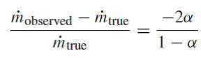
where![]() is the mass flow rate and
is the mass flow rate and ![]() is the GVF on a scale of 0 . . . 1. The density error simply takes the form
is the GVF on a scale of 0 . . . 1. The density error simply takes the form
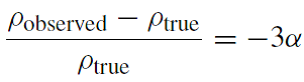
where ![]() denotes density. Note that although in the above equations GVF is on a 0 . . . 1 scale, it is more frequently considered on a percentage 0 . . . 100% scale, which will be used for the remainder of the text. For clarity, it is to be understood that in this simplest of models the mass of the gas is assumed to be negligible, and hence the nominal mass flow of the two-phase mixture is equal to the mass flow of the liquid phase only. However, when assessing the density error, it is more useful to consider the meter’s ability to measure the density of the two-phase mixture rather than of the pure liquid itself. Thus, with a liquid density of (say) 1000 kg/m3 and a GVF of 10% , assuming the gas has negligible mass, the nominal mixture density is 900 kg/m3. In these conditions, a density error of say −5% would mean that the meter was reporting a mixture density of only 855 kg/m3.
denotes density. Note that although in the above equations GVF is on a 0 . . . 1 scale, it is more frequently considered on a percentage 0 . . . 100% scale, which will be used for the remainder of the text. For clarity, it is to be understood that in this simplest of models the mass of the gas is assumed to be negligible, and hence the nominal mass flow of the two-phase mixture is equal to the mass flow of the liquid phase only. However, when assessing the density error, it is more useful to consider the meter’s ability to measure the density of the two-phase mixture rather than of the pure liquid itself. Thus, with a liquid density of (say) 1000 kg/m3 and a GVF of 10% , assuming the gas has negligible mass, the nominal mixture density is 900 kg/m3. In these conditions, a density error of say −5% would mean that the meter was reporting a mixture density of only 855 kg/m3.
Although the bubble model is successful in predicting the general characteristics of two-phase flow errors (i.e. negative and increasing in magnitude with GVF), the pattern of errors observed experimentally are much more complex, at present poorly understood, and vary
with a number of different parameters.
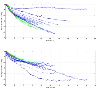
Figure 1. Mass Flow and Density errors for air/water mixes, 75mm flowtube.
Experimentally observed two-phase flow errors for air-water mixtures
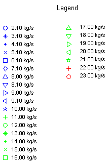
The UTC has investigated two-phase flow errors using a variety of flow-tube designs and fluids. Their experience suggests that while for low viscosity fluids the negative errors predicted by the bubble model form a good first approximation of the experimentally observed errors, there are additional influencing factors which the model excludes. The underlying assumptions of the model – which include no interaction between bubbles, and no interaction between the bubbles and the flow-tube wall – are clearly not applicable in many circumstances, for example with slugging flow. One observation from experimental data is that, even at relatively low GVFs where the bubble model should be closest to reality, there is a high dependency of mass flow error on the mixture velocity. This is illustrated in Fig. 1, which show for a 75 mm flowmeter, the mass flow and density errors as they vary with both GVF and mass flow with water as the liquid component. These results were obtained at an industrial flow laboratory with instrumentation traceable to NIST, using equipment and procedures similar to those described later in the paper. At low GVF, say 5 %, the mass flow error can vary from -9 % down to -20% as the flow rate ranges from 23 kg/s down to 3 kg/s.
Factors other than GVF and mass flow affecting the measurement errors include the following:
Flow-tube orientation.
Changing the orientation of the flow-tube (e.g. from horizontal to vertical positioning) results in different error curves. This suggests a role for buoyancy forces in the mass flow and density errors.
Flow-tube geometry.
The complex geometry of a “bent” flow-tube might reasonably be assumed to influence the effects of two-phase flow. However, straight tube geometries are also found to exhibit similarly complex error curves. In each case, different flow-tube geometries produce somewhat different errors. Similar flow-tubes of different sizes (e.g. the same commercial offering with different diameter tubes) appear to produce similar, but not identical (scaled) error curves. Features such as whether the tube is split or continuous path are clearly significant.
Process fluid viscosity and other properties.
Viscosity is a significant contributory factor, as perhaps are other fluid properties and application conditions. An extended version of the bubble model which incorporates viscosity effects suggests that, as the viscosity tends to infinity, both mass flow and density errors tend to zero [3].
Transmitter effects.
As discussed in [4], even if flow-tube oscillation is maintained, unless the flow-tube frequency and phase are tracked very carefully and matched in the drive signal, the result may be forced rather than natural oscillation, introducing (in our experience) random walk in the observed phase measurement, which is non-stationary and hence difficult to correct.
To summarize, the accumulated experimental experience using many flow-tubes and fluids suggests that the mass flow and density errors are generally smooth (with respect to flow rate and GVF) and negative. The exact forms of the curves are dependent on a number of complex factors, including orientation and flow-tube geometry, which are presently not readily amenable to theoretical analysis.
Two-Phase Flow Correction Methodology
The definition of two-phase flow correction used here is the application of compensation to the raw mass flow and density readings for the effects of two-phase flow, in order to generate improved (corrected) readings, where the correction is based solely on data available within the flowmeter. It is however reasonable to allow single-valued configuration parameters (such as the nominal single phase liquid density, perhaps with a temperature coefficient of expansion) to be provided by the user.
The means of two-phase correction is some form of model which predicts, from configuration data and on-line internally-observed parameter values, the required corrections to the raw mass flow and density values. While a universal correction model based on physical principles would be ideal, the current state of knowledge is far from complete. However, there is an accumulating body of experience which indicates that, for a specific flow-tube geometry and process liquid, within a reasonable range of application conditions (e.g. flow, temperature, pressure), empirical on-line correction models can provide substantial improvements on the uncorrected measurements.
To develop a model, an experimental grid of test points is defined, covering a range of flowrates and GVFs. Controlled variation in other conditions, such as inlet pressure and temperature, may be included in the experimental grid. Typically in such experiments, Coriolis meters are also used to to provide reference measurements of the single phase liquid and gas streams before they are mixed and subjected to the test meter, so that the single phase component flow rates have typical uncertainties of 0.2 % for the liquid and 0.5 % for the gas stream. At each experimental point, internal parameters are recorded and averaged over a pre-determined time period (typically 30-120s, selected to ensure a representative sample of the two-phase flow conditions) for use in model fitting. Given independent measurement of the true single phase flows of the liquid and gas phases, and assuming (or engineering) good mixing between the phases (i.e. no slip), it is possible to calculate the true mass flow and (mixture) density, and hence to calculate the corresponding errors in the raw measurements. Additional instrumentation is required to provide pressure and temperature information for the single phase gas and for the mixture, to enable PVT calculations of gas volume in the mixture and hence void fraction. Note that as pressure drop occurs across the flow-tube, the GVF is not constant, but increases through the meter. By convention, therefore, GVF is calculated based on the pressure at the inlet to the flow-tube.
A number of different model-fitting techniques might be used to predict the mass flow and density errors based on the internally observed parameter values, but the UTC has found the use of neural nets to be satisfactory. The resulting neural net models can be run on-line to apply corrections to the raw mass flow and density readings in the presence of two phase flow. Examples of the types of parameters, and the neural net modelling applied, are described in [5]. As demonstrated in the following example, this approach has delivered effective error reduction.
In the case of the 75 mm flow-tube with water, whose mass flow and density errors are shown in Fig. 1, on-line correction models have been developed and applied. Fig. 2 shows the residual errors observed in separate trials at the same facility with the correction applied on-line. The tests of the corrected data were all carried out within the experimental grid of the model data (mass flow between 5 kg/s and 20 kg/s, GVF < 25 %, inlet pressures between 0.3bar and 1.1bar, temperature between 27.8C and 32.3C), and hence the neural nets are interpolating rather than extrapolating. Additional techniques have been developed to deal with extrapolating beyond the known region. The resulting errors are fairly typical of two-phase correction achieved using this methodology, with the density proving particularly amenable to correction, while the corrected mass flow manifests higher error scatter. For density, approximately 95 % of the experimental points for all GVFs have error magnitudes less than 0.4 % (for other flow-tubes and liquids a more typical value is 1 %). There is greater spread for the corrected mass flow reading. For GVFs less than 10 %, 95 % of the errors are less than 2 %, while for all GVFs the 95 % probability error is approximately 4 %.
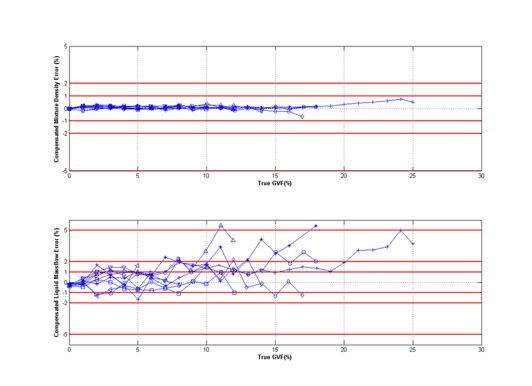
Figure 3. Corrected mass flow and density measurements - independent trials
References
[1] Reizner, J.R. “Batch accuracy: the good, bad and ugly of Coriolis”, InTech Magazine, March 2005.
[2] Hemp, J. and Sultan, G, “On the theory and performance of Coriolis mass flow meters”. International conference on mass flow measurement; direct and indirect, Coriolis metering I. London 21-22 Feb, 1989. Organised by IBC Technical Services Ltd.
[3] Hemp, J and Yeung. H. “Coriolis Meter in Two Phase Conditions”, IEE Seminar on Advanced Coriolis Mass Flow Metering Ref No.03/10224. Oxford, 2003.
[4] Henry, M. P., Duta, M. D., Tombs, M.J., Yeung, H., Mattar, W. “How a Coriolis mass flow meter can operate in two-phase (gas/liquid) flow”, ISA Expo Technical Conference, 2004.
[5] Liu, R. P., Fuent, M. J., Henry, M. P. and Duta, M. D., “A neural network to correct mass flow errors caused by two phase flow in a digital Coriolis mass flowmeter”, Flow Measurement and Instrumentation. March 2001; 12(1): 53-63.